A 200-Case Test Changed the 3D Surrogate Ranking

I was comparing models that approximate airflow and temperature in a demonstration room. One used Proper Orthogonal Decomposition (POD) to compress simulated fields into shared patterns, then Gaussian-process regression (GP) to predict their weights. The other, NVIDIA PhysicsNeMo’s Fourier Neural Operator (FNO), learned the field mapping directly.

The first 3D comparison looked decisive. At 240 training snapshots, POD+GP scored 8.45% mean field error and the FNO scored 11.30%. I wrote that the classical method led by two to three points, then started explaining the lead in terms of limited data and the relative efficiency of a reduced basis.

Both models had been judged on only 16 held-out room cases. I was explaining an unstable comparison.

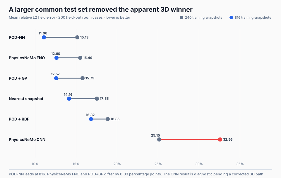
When I scored them again on one common set of 200 cases, the Gaussian process moved to 15.79% and the FNO to 15.49%. The apparent winner reversed. At 816 training snapshots they reached 12.57% and 12.60%, a difference of three hundredths of a percentage point in this recorded run. I do not have repeated FNO seeds or a predefined equivalence margin, so I treat them as numerically adjacent rather than statistically tied.

The small test set had not added equal noise to both methods: compared with the 200-case test, it flattered the Gaussian process by a factor of 1.87 and the FNO by 1.37, so the gap I was explaining was almost entirely an evaluation artifact.

This article takes the technique question from Part 3’s five 2D problems into 3D: what changed in the solver, how the comparison was corrected, and why a close score still leaves a real technique choice. Part 2 records what the public repository includes and excludes.

3D changed more than the array shape

The 2D room uses a streamfunction-vorticity formulation. There is no equivalent scalar streamfunction for this 3D flow, so the 3D demonstration solver uses primitive velocities and a fractional-step pressure projection. In the measured profile, the pressure Poisson solve consumed 51% of wall time.

The output changed from three fields on a section to four fields in a volume, so at a 24-cubed grid one snapshot contains 55,296 values across three velocity components and temperature, while the input gains diffuser width, a geometric parameter with no 2D equivalent. Nothing else stayed equal.

Those changes do not affect every surrogate family in the same way. POD flattens each snapshot into a matrix column, so the linear algebra does not care whether a value came from an image or a volume, although storage grows with the field. An FNO performs spectral operations over the spatial dimensions themselves. Its spectral weight count grows with modes^dimension, which makes a copied 2D configuration expensive in 3D.

The PhysicsNeMo FNO API supports 1D through 4D fields. Support didn’t make the 2D configuration sensible for this dataset, so I capped the 3D path at six modes, width 16 and two layers rather than fitting the much larger 2D defaults to a few dozen snapshots.

I used the actual physicsnemo.models.fno.FNO import for the PhysicsNeMo row. The hand-written PyTorch FNO in the workbench remains a separate technique. A vendor library, a model architecture and my data-conditioning wrapper are different parts of the execution path, and the report now names them separately.

The common test changed the ranking

The data didn’t come from an external dataset. I generated it with SurrogateLab’s built-in demonstration 3D room solver through the command-line entry point gen_3d.py. The web interface can launch the same generator, but the browser doesn’t generate the fields itself. That run produced 1,000 training cases and 16 original test cases.

For the corrected comparison, I pooled all 1,016 cases, used seed 0 to hold out one common set of 200, and formed nested 240- and 816-case training sets from the remainder. The 240-point set was contained inside the 816-point set, so every technique and both data budgets had to answer the same held-out questions.

The retained code and result summary document this comparison, but the exact generated NPZ arrays were not found in the local archive reviewed for release. I cannot replay these exact scores locally without them. Regenerating the dataset would be a new reproduction run, not a recovery of this one.

I also checked the nearest-snapshot baseline, whose mean field error fell from 17.55% to 14.16% as the training set grew. That is an observed improvement, not a property the split must guarantee. The implementation chooses the nearest training input; a closer input can still give a worse field prediction. With a fixed input-distance metric, adding training points cannot increase the nearest input distance, but field error need not follow it. The common test and nested sets make the comparison more controlled; a falling baseline does not prove the split is correct.

POD-NN overtook POD+GP at 240 snapshots and kept a 1.51-point lead at 816. I was wrong. The same small joint coefficient regressor that failed on the thin 2D moving-diffuser case now had enough examples to improve on the independent per-mode Gaussian processes. I would not turn the crossover into a universal sample threshold; the retained mode count also grew from 51 to 186 as the dataset became more diverse.

At 12.6%, the remaining choice is operational

PhysicsNeMo FNO and POD+GP arrived at roughly 12.6% by different routes in this run.

The FNO had 886,172 learned parameters and took 291 seconds to train in the recorded run. The POD basis stored 10,285,056 values and the complete POD+GP fit took 4.3 seconds. The neural operator used about twelve times fewer stored numbers and took about 68 times longer to produce them.

That makes the choice operational rather than ideological. I would look at POD+GP when the model has to be rebuilt often as new reference cases arrive and storage is cheap. I would investigate the FNO when package size matters enough to justify GPU training. Field-resolution transfer can be an FNO advantage, but this fixed-grid experiment didn’t test it. POD-NN is the awkward result for both narratives: it was smaller in implementation, needed no PhysicsNeMo dependency, and had the lowest error in this test.

The wider PhysicsNeMo model catalogue includes graph, point-cloud, voxel and neural-operator approaches that are more natural for large 3D CAE problems than this compact FNO experiment. This run does not compare those architectures. It shows that importing a current framework does not decide the method, and that a classical baseline can remain competitive on a small parametric dataset.

The CNN row is a failed path, not a result to generalise

The PhysicsNeMo Pix2Pix convolutional encoder-decoder improved on some 2D problems and tied for best on energy. In 3D it reached 25.15% at 240 snapshots and 32.56% at 816 while every other technique improved.

The first implementation did not include absolute coordinate channels, a serious omission for a room where ceiling and floor are physically different. I added them, expecting the larger run to recover, but it still degraded; that rules out one suspected cause and leaves the current 3D conditioning or training path under question.

I am keeping the row in the chart because it is useful diagnostic evidence. I am not using it to say convolutional surrogates get worse with data, or that the PhysicsNeMo architecture is at fault. This implementation hasn’t earned an accuracy claim until the path is corrected and rerun.

The parameter box changed the headline too

The 3D sweep found another problem that the 2D room hid. Above a Richardson number of roughly 3.5, about 10% of the original parameter box didn’t settle to a steady solution. The buoyant plume and the supply jet continued to oscillate. A steady surrogate can’t learn a steady answer that doesn’t exist. The main common-test table includes the original pool, including those cases. A separate diagnostic compared the full box with a well-posed region.

Those cases were between 3.0 and 3.8 times harder for the tested techniques and added 19% more POD modes for 10% more data. Excluding them from training improved all four methods in that diagnostic by 1.2 to 3.9 percentage points. Mean error over the well-posed diagnostic was about 7%; including the non-steady region pushed it toward 12%.

That is one re-partition of one demonstration dataset, so I would not reuse its percentages as a general CFD rule. I would reuse the question: before fitting a steady surrogate, verify that the reference problem has a steady solution throughout the declared operating box.

What I changed after the 3D runs

I no longer accept a sample-count ladder built from a different held-out set at each rung. I keep unavailable or failed methods in the reports because deleting them would erase the route by which I found the comparison defects. I also separate official PhysicsNeMo imports from models that only share an architecture name.

Most of all, I stopped treating 3D as a larger confirmation of the 2D ranking. It changed the reference solver, exposed a non-steady regime, shifted the model economics and removed a result that had looked obvious on 16 test cases.

Part 5 returns to the building use case. It asks whether these field errors and millisecond predictions are enough for a comfort decision, rather than whether they are enough to win a benchmark table.

Disclaimer: The views and opinions expressed in this account are those of my own and do not represent those of my employer, NVIDIA.