What It Would Take to Put a Room Surrogate in a Comfort Loop

I spent part of my early career putting closed-loop control into refineries. A process model could choose the next move, but that didn’t make it responsible for plant safety. We kept safety in separate layers because the model could be wrong. I came back to that commissioning boundary when I looked at the ventilated-room surrogate.

The workbench was fast enough to compare ventilation choices interactively. But when I checked quantities in the occupied zone, the model with the lowest whole-field error did not lead every comparison. I could not choose a model for a comfort decision from that overall score alone.

SurrogateLab demonstrates the fast prediction path and exposes several of the right checks. It hasn’t yet established a comfort model that I would connect to a live building. Part 2 describes the repository’s public scope and evidence boundary.

What the current model can show

The demonstration room has a supply opening near the top of one wall, a return near the bottom of the other and a heated floor. Its parameters vary supply momentum, buoyancy and opening size; the 3D version also varies diffuser width. The reference solvers produce velocity and temperature fields, and the surrogate learns those fields over the sampled box. The two captures below use POD+GP and the currently retained 2D dataset so their source can be inspected and rerun.

That stored test set contains 26 cases. The truth-versus-surrogate animation selects 16 of them for a readable sequence; the comfort table later in the article scores all 26.

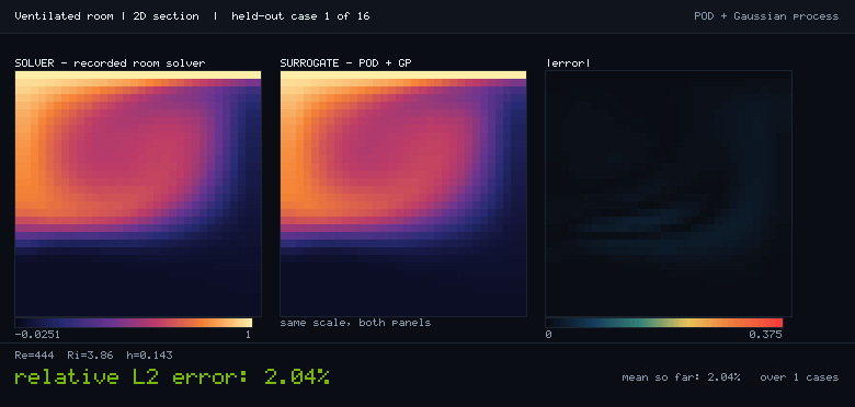
One held-out case makes the output tangible:

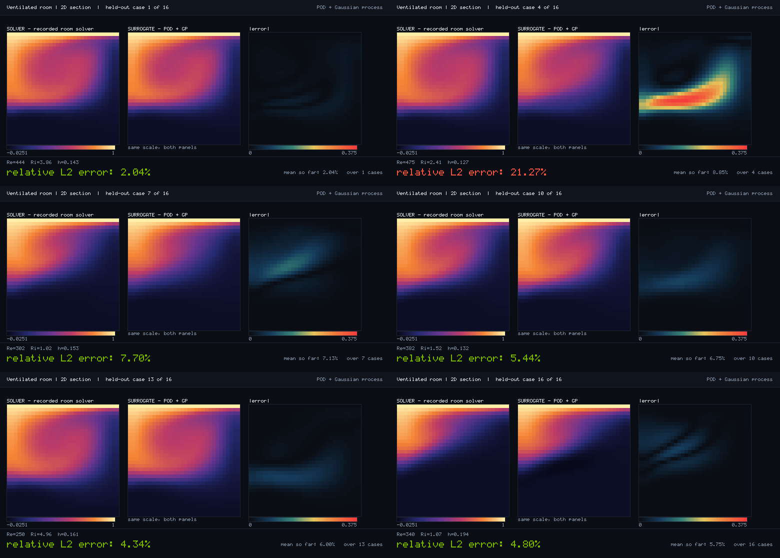
Show the 16-case animationHide the animation

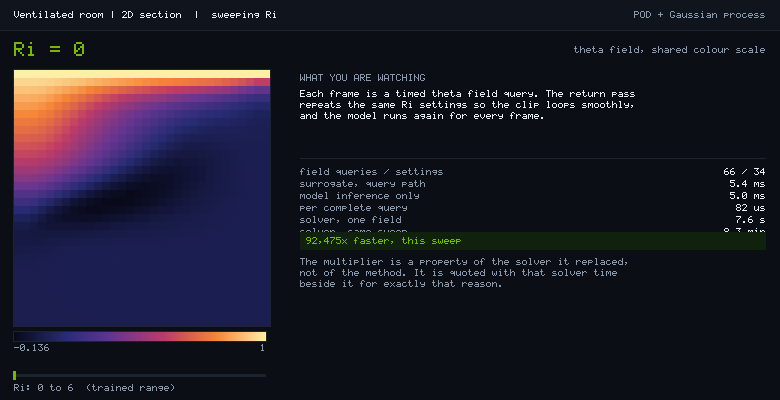
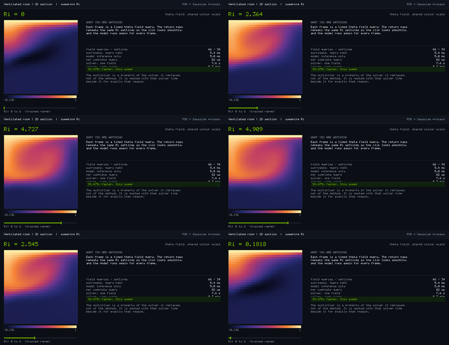
The fast path matters when the question is repeated. The corrected sweep executes 66 timed field queries across 34 distinct Richardson-number settings. The outward pass visits each setting once. The return pass repeats the interior settings so the clip loops smoothly, and the model runs again for every frame. The complete surrogate query path took 5.4 milliseconds for all 66 calls in this capture. The model’s internal inference timing accounted for 5.0 milliseconds of that total; neither number includes rendering the GIF.

The reference comparison is an extrapolation, not 66 newly executed solver runs. The retained dataset records a 7.5818-second mean reference-solve time on the machine used for generation. Multiplying that value by the same 66 queries gives 500.4 seconds, which the animation displays as 8.3 minutes.

Show the parameter-sweep animationHide the animation

That makes the repeated comparisons from Part 1 practical: someone can try another ventilation setting without waiting for a fresh reference solve. The reference solver is still needed to check the approximation.

The field winner was not the decision winner

I evaluated four models on the 26 held-out cases in the stored 2D room dataset, then compared the mean absolute error for each derived quantity with the standard deviation of that quantity across the test set. In this table, 0.18 means the model’s mean absolute error is 18% of the held-out variation; it does not mean 18% error in temperature or speed.

POD-NN is still a good whole-field result. It is also the wrong default if vertical gradient is the condition that decides the action. The Gaussian process and RBF interpolate each modal coefficient independently, yet both preserve that particular derived quantity better on this test. I nearly turned the table into another technique explanation, but I don’t have enough evidence to assign a general mechanism to the difference; I have enough to stop ranking a comfort surrogate by one field norm.

This table is not an engineering acceptance test. It is two-dimensional, uses non-dimensional demonstration fields and has only 26 held-out points. It does show how a technique comparison changes once the output is tied to a decision.

A real comfort decision needs more than these fields

ASHRAE Standard 55 treats comfort as a combination of environmental and personal factors. Air temperature and air speed matter, but so do mean radiant temperature, humidity, clothing and activity. Local discomfort adds effects such as draft and vertical temperature gradient.

The workbench has velocity, temperature and a few derived occupied-zone quantities. It doesn’t model humidity, radiant exchange, clothing, metabolic rate or a validated turbulence field. Its coarse laminar solver hasn’t been checked against a measured room. A surrogate that reproduces it closely is still an approximation of an unvalidated reference.

The two-dimensional section carries another limit. It has no end walls, corners or spanwise velocity, and its plane jet decays differently from a diffuser in a volume. The 3D demonstration is closer to the shape of the question, but it remains a coarse fixed-geometry study. Part 4 also found that part of the original 3D parameter box had no steady solution, which means a steady surrogate can’t cover that region honestly.

I would describe the current evidence this way: it is enough to demonstrate a ventilation what-if loop and to test surrogate methodology. It isn’t enough to claim compliance, predict occupant satisfaction or command a building.

How I would place it in a smart-building twin

I would keep two prediction paths rather than replace every building model with a surrogate.

The energy row is deliberate. I assumed every large speed-up was supporting evidence for a surrogate, but in the workbench the compact energy calculation takes roughly a tenth of a second; making it 655 times faster doesn’t improve a nightly calculation or a small scenario set if nobody is waiting, so I would run that model directly and reserve approximation for the spatial CFD path that blocks interaction.

The answer can change with scale. A portfolio study that multiplies buildings, retrofit combinations, weather years and control policies may turn a fast energy model into the workload bottleneck. The complete workload test from Part 1 still applies; the use-case label does not choose the architecture.

The release gates for operational use

Part 1 asked whether the workload justifies building a surrogate. These gates ask whether an existing surrogate can influence an operational choice. Before this moved beyond a demonstration, I would require six additions.

1. A validated 3D reference. Use an engineering CFD setup with a mesh study, an appropriate turbulence treatment and comparison against a measured or accepted benchmark room.
2. Operational inputs in physical units. Map BMS points, weather, occupancy, glazing load and actual control commands into the model. Reject states that cannot be mapped inside the trained domain.
3. A complete comfort calculation. Add the environmental and occupant factors required by the intended comfort method, rather than treating temperature and velocity as the complete answer.
4. Common held-out decision tests. Set acceptance thresholds for occupied-zone quantities and constraint violations, including p90 and worst cases, across the final operating box.
5. A governed fallback. Route out-of-domain, uncertain, drifted or consequential cases to the reference solver or to a conservative operating policy, and retain the reason.
6. A staged building trial. Start in shadow mode, then advisory mode. Compare predicted and observed response before the model is allowed to close a control loop.

The current project clears only part of that path. It has a measurable latency advantage, enforced parameter bounds, held-out field tests, comparison against a trivial baseline and retained reports. Its 3D comfort quantities, reference validation, live state mapping and observed-building feedback remain open.

Disclaimer: The views and opinions expressed in this account are those of my own and do not represent those of my employer, NVIDIA.