Building SurrogateLab: The Workbench Behind SurrogateGate
Pradeep Kaushik·Sep 7, 2026·Build Note·12 min read·Updated Sep 21, 2026
In this article 8 sections
When repeated simulations miss an application’s decision deadline, could an approximation answer fast enough without changing the decision? I built SurrogateLab to compare the candidates, then found that the comparison itself needed repair.
The main applied case was predicting a room’s airflow and temperature under different operating conditions. The first large report grouped 76 current, repeated and superseded runs on one page. I was reading a trend into rows that should not have been compared. The sample-count ladder also changed the held-out cases at each rung, so the scores could move because the test changed, even before I considered what more training data had done.
Part 1 asks whether an approximation is needed at all. This build follows the next question: how to give competing methods a fair test before choosing one.
A catalogue of algorithms couldn’t answer that. A Gaussian process, a reduced-order model, a neural operator and a physics-informed network make different assumptions and consume different amounts of data and compute. A method that works well on a fixed 2D field may not be right for a 3D case, and a low average field error may still hide a wrong decision quantity.
I call the broader project and decision framework SurrogateGate. SurrogateLab is the executable workbench and the name carried by its code, reports and public repository. This article follows the workbench.
I needed scenarios where the answer could be no, a trivial baseline that sophisticated methods could lose to, separate two- and three-dimensional tests, and reports that retained failed or unavailable methods.
I brought a controls habit to the workbench: ask where a model was tested, how I’ll know it has left that range, and what happens next. A benchmark report that answers only “which row is lowest?” isn’t enough for an operational twin.
What a fair result has to retain
In the original 3D ladder, increasing the training budget also changed the held-out questions. A trend across those rungs could not distinguish the effect of more data from the effect of a different test.
I completed the common-test correction with internally generated data. SurrogateLab’s built-in demonstration 3D room solver produced it through gen_3d.py; no external dataset was involved. The run produced 1,000 training cases and 16 original test cases. I pooled all 1,016, used seed 0 to hold out 200 once, and drew nested 240- and 816-case training sets from the remainder. That removed an apparent two-to-three-point advantage for a classical reduced model (POD+GP) over a learned field model (the PhysicsNeMo Fourier Neural Operator, or FNO). The larger experiment did not finish every question: the complete catalogue still lacks a multi-seed distribution, and the 3D convolutional network (CNN) path remains diagnostic after its accuracy degraded with more data.
These are the checks I use to judge the comparison. The common test and nested training sets are in place; repeated seeds and reference-data validity still have gaps, so this is not a list of completed validations:
One common held-out test set across data budgets. The earlier sets can compare techniques within one run, but not establish a training-volume effect across runs.
Nested training sets for a sample-count ladder. A larger rung should contain the smaller rung plus additional points. Otherwise data volume and sample placement are confounded.
The same parameter box and preprocessing. Input ranges, field scaling, retained-energy rule and reference-solver version belong to the experiment definition.
A trivial baseline in every table. A complex method that does not beat the nearest stored solution has not earned its complexity.
Mean, tail and worst-case error. Averages can hide the exact operating corner a user cares about.
Decision quantities as well as whole-field error. For ventilation that means occupant-zone temperature, velocity or comfort-relevant quantities, not only one aggregate norm over the room.
Separate solver, training and inference time. A speed-up multiplier without the measured solver time beside it says little, and training cost matters differently from per-query latency.
Several seeds where optimization is stochastic. This remains incomplete for parts of the catalogue, so small neural gaps stay provisional.
Convergence and validity status for every reference run. A surrogate cannot repair a reference field that never reached the state the experiment says it represents. The main 3D comparison still uses the original pool, including its non-steady region; Part 4 explains that limitation.
The diagnostic before the leaderboard
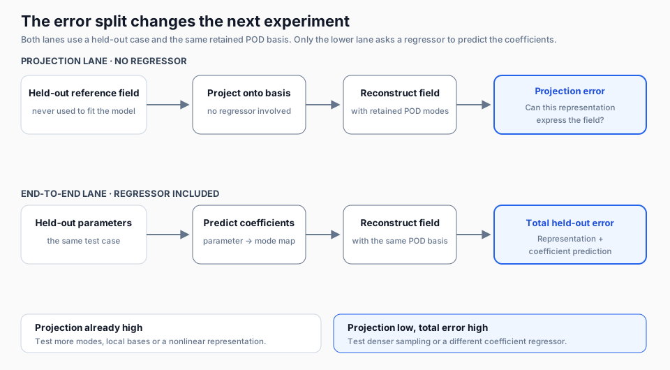
Proper Orthogonal Decomposition (POD) compresses spatial fields into a set of shared patterns, or modes. A regressor predicts how much of each mode to use for a new set of inputs. Before choosing a more complex method, I need to know which of those two steps is failing.
Projection error asks whether the retained basis can represent a held-out field. I project the reference field directly onto the basis and reconstruct it without using the regressor.
Regression error is the remaining gap introduced when the model has to predict the modal coefficients from the input parameters.
I added the upper lane after realizing that one total error number did not tell me what to change. It separates a representation problem from a parameter-map problem before I reach for a larger model.
If projection error is already high, I test more modes, local bases or a nonlinear representation. If projection is low but total error remains high, I test denser sampling, a different regressor or joint coefficient prediction. Looking only at the singular-value spectrum sees the first problem and can miss the second. Looking only at total error says something is wrong but not what to change.
That diagnosis is more useful to the next experiment than a winner at one data budget. It tells me whether to change the representation, collect more samples or inspect a decision metric that exposed a localized miss.
A workbench built around gates
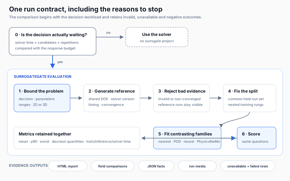
The first branch is part of the workbench, not a preface to it. A scenario can stop with the original solver. When it continues, every technique receives the same evidence and the negative rows remain in the report.
I placed technique selection after the need, scope and evidence gates. If the reference model is already fast enough, the run says so. If a steady solver didn’t converge, I don’t want that snapshot quietly entering the training set. If a method is unavailable because a dependency or GPU is missing, the comparison keeps the row and the reason.
The workbench currently separates the interface from the modeling library: the library owns solvers, sampling, reduction, fitting, validation, decisions and durable run records, while the browser guides a user through the choices and makes the result inspectable. Batch mode executes that same path across several configurations and builds a cross-run comparison.
I use the same path for an individual demo and the larger experiment so they can’t quietly acquire different definitions of success.
The interface matters because the gates are meant to interrupt an easy slide from “I can fit a model” to “the model belongs in the runtime loop.” This walkthrough follows one retained 2D ventilated-room run through the actual workbench.
The 80-second silent walkthrough condenses two screen recordings and plays the interaction at twice its original speed. It moves from problem selection through scope, generated evidence and technique choice, then compares several surrogates with one solver result before opening the field render and retained report. The row values belong to this demonstration run; Parts 3 and 4 use the corrected comparison records.
The report is part of the experiment
Each run produces more than a score: the current HTML report retains the selected problem, dimensionality, data budget, technique availability, held-out metrics, timing, field comparisons, the conclusion reached by each gate and a machine-readable JSON record. Batch reports place several runs into one comparison surface.
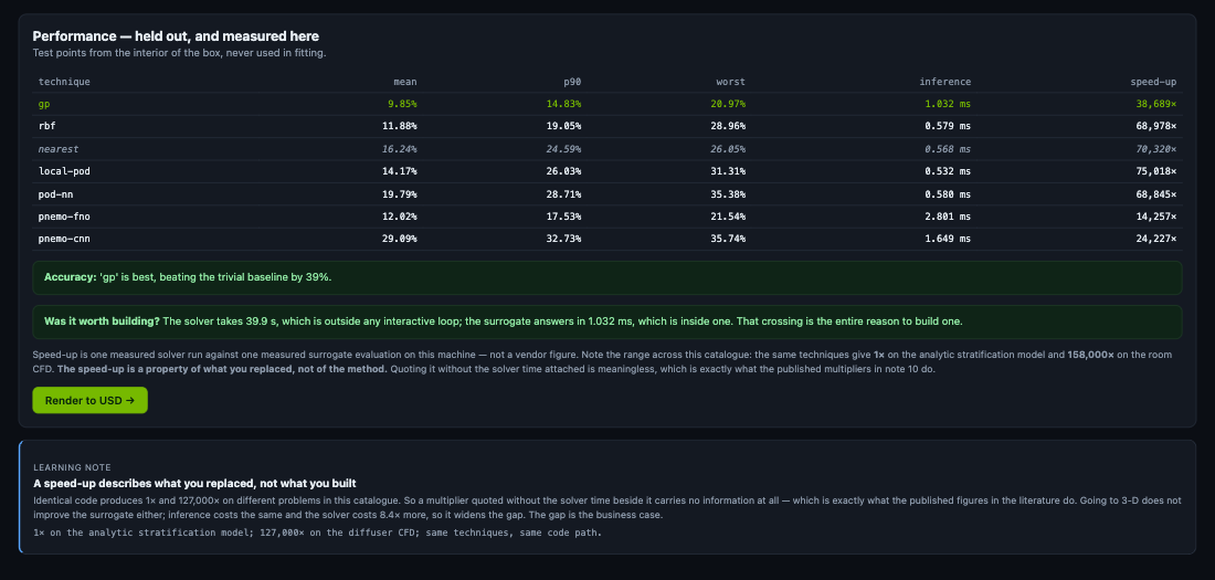
One 3D run shows the report surface I wanted: the trivial baseline, tail error, inference time and measured solver time remain beside the technique rows. The rows are comparable within this run; this image does not establish a sample-efficiency ranking across runs.
The report retains field comparisons, parameter sweeps and embedded facts so article figures can trace back to a run. That trace still needs checking.
I initially treated a retained historical aggregate HTML page as a sampling-trend report. That was a mistake. It combines 76 run cards, including repeated configurations and superseded experiments, and its old trend grouping could join runs that did not use the same underlying dataset. One summary sentence also retained the old claim that the small 3D test flattered the GP by a factor of 2.00; the corrected common-test calculation is 1.87. The current generator treats the aggregate page as a run index and does not infer a trend across those records.
Individual HTML reports preserve the configuration and comparisons within a run. The older PDF batches predate the common 3D test and include superseded 2D values, so I excluded them as source figures for the series.
An adversarial pass found a separate defect in the parameter-sweep capture. The old clip predicted 34 fields, displayed 66 frames by reusing them in reverse, and compared that work with 66 solver evaluations. I corrected the generator and added a regression test. The new 2D room clip executes 66 timed field queries across 34 distinct settings, including a newly evaluated return pass. Its accompanying truth sequence selects 16 cases from the retained 26-case test set. Part 5 keeps the measured and extrapolated quantities explicit.
Five problems chosen to produce different answers
My first design requirement was disagreement. A benchmark made only from surrogate-friendly cases would teach me how to tune a demo, but not when to stop.
The current catalogue uses five deliberately different building-related problems:
Scroll sideways for more columns.
Problem
What changes
What it tests
Ventilated room
Flow, buoyancy and supply conditions
A fixed-geometry field problem connected to local comfort
Moving diffuser
A supply location changes as part of the input
Whether geometry-like movement strains a shared representation
Contaminant dispersion
A transported scalar forms a spatial plume
How a localized or moving feature affects representation and regression
Whole-building energy
Operating parameters drive energy outputs
The counterexample: a solver may already be fast enough for the intended loop
Displacement stratification
A compact analytic relationship produces the response
A control case where approximation overhead can be harder to justify than direct evaluation
The ventilated room is the main applied thread. It has a credible decision question about local comfort under alternative operating conditions, and it produces spatial outputs that make technique differences visible.
I kept the energy and stratification cases because a surrogate can be accurate and fast yet still be unnecessary. “Large speed-up” does not establish value if the original calculation already met the application’s response budget.
These are demonstration problems, not validated engineering models. The CFD implementations are intentionally compact, use coarse grids and do not establish accuracy against a measured room. Every surrogate error in this project is therefore surrogate versus the selected reference solver, not surrogate versus reality.
The comparison is between technique families, not labels
The workbench includes techniques from several families. I keep the family and implementation provenance visible because I found that the display name could imply a comparison the code had not actually run.
Classical reduced models
The classical path uses Proper Orthogonal Decomposition, or POD, to compress a set of spatial fields into modes. A regressor then maps input parameters to the coefficient of each retained mode.
The current choices include:
Nearest snapshot returns the closest training example and acts as the minimum baseline.
Radial basis interpolation is a small and inexpensive interpolator.
Gaussian-process regression adds a probabilistic model of the coefficient map.
Local POD allows more than one linear basis over the input space.
POD-NN is a small neural regressor that predicts the same POD coefficients jointly.
POD-NN is a particularly useful control. It keeps the POD representation fixed and changes only the parameter-to-coefficient map. If it improves on POD plus GP under the same split, the result points toward regression capacity rather than a failure of the linear basis.
Learned representations and neural operators
I use the second group to change more of the pipeline. It includes an autoencoder, a plain PyTorch Fourier Neural Operator and other neural experiments that learn a representation or the field mapping more directly.
These models introduce more capacity, more training choices and usually a greater appetite for data. I’m not testing whether they can fit the training set. I’m testing whether they improve held-out decisions enough to justify those costs.
PhysicsNeMo implementations
The project also includes official NVIDIA PhysicsNeMo-based FNO and convolutional implementations. I gave them distinct keys from the hand-written PyTorch models so the reports show which library actually ran.
PhysicsNeMo broadens the techniques available for physics-ML work. The pnemo-fno and pnemo-cnn rows in this project are supervised on solver fields. The separate PINN row adds an equation residual. The framework import does not make every model physics-informed, and a physics term in the loss does not guarantee conservation or operational safety. Every row still has to beat the nearest-neighbour and classical baselines on the same held-out data.
2D and 3D are separate tests
The workbench supports a 2D room section and a 3D room, but I don’t treat 3D as a resolution setting.
The 2D reference uses a streamfunction-vorticity formulation. In 3D the workbench uses primitive variables and a fractional-step method with a pressure solve. That difference changes both the physics that can appear and the cost of generating reference data.
The surrogate families feel the change differently:
Scroll sideways for more columns.
Technique property
Moving from 2D to 3D
POD after field flattening
The spatial vector becomes much larger, but the reduction still operates on a snapshot matrix
Coefficient regressor
The input dimension may stay small even when each raw output field becomes much larger
Grid-based neural operator
The network now operates over another spatial dimension, changing memory and spectral-layer cost
Convolutional field model
Training tensors and activations grow with the volume
Reference-data generation
The 3D solver may use a different numerical scheme and costs more per snapshot
I use the 2D suite for broad, cheaper comparison and faster correction of the test harness. The 3D suite then asks whether those findings survive a larger output, a different solver and different scaling behavior.
Part 3 reports the corrected 2D comparisons. Part 4 treats the 3D and PhysicsNeMo evidence separately; a 2D win does not establish a 3D conclusion.
What the project establishes today
The SurrogateLab repository is now public as a research preview. Generated data, checkpoints, local run records and media remain excluded. The repository includes an MIT license, third-party notices and a sanitized evidence summary that states what cannot be reproduced from the retained files. Its test and privacy checks passed before publication. It does not establish a universal winning technique or an engineering-valid comfort model. It does establish a controlled sample-volume result for this one 3D room, while the stochastic methods still need repeated seeds before small gaps should be treated as stable.
Part 3 uses the workbench to compare five 2D problems. Part 4 repeats the 3D comparison on a common test set. In Part 5, I check whether the results are useful for a comfort decision and where a solver fallback is still needed.
Disclaimer: The views and opinions expressed in this account are those of my own and do not represent those of my employer, NVIDIA.