When a surrogate predicts the wrong temperature or airflow field, I need to know what to change. Can its compressed representation describe the field at all, or is the learned mapping from room conditions into that representation the weak point? I used five 2D demonstration problems to separate those questions before choosing a more complex model.
The moving-diffuser case made the distinction clear. Moving the supply opening changes where the flow enters the room. The compressed representation could reconstruct the held-out fields well when given their known coefficients, but predicting those coefficients from the inputs introduced much more error. The result table below shows how differently the tested methods handled that mapping.
This is the 2D evidence from the SurrogateLab workbench in Part 2, which also records what the public repository includes and excludes. Every error below compares a surrogate with a demonstration solver. I haven’t validated that solver against a measured building. The retained ventilated-room dataset has its own 26-point test set. Each of the other four rows comes from the four-problem catalogue batch, with a separate 26-point held-out draw for each problem. Those rows support comparisons within each problem. Reading them as one shared cross-problem batch would overstate the evidence, and the absolute rankings remain specific to these datasets and implementations.
The results I now use
Proper Orthogonal Decomposition (POD) compresses fields into a set of spatial patterns, or modes. POD+GP predicts their coefficients with Gaussian-process regression; POD-NN uses a neural network. A Fourier Neural Operator (FNO) learns the field mapping directly. The projection-error column tests the POD representation without asking a regressor to predict its coefficients.
Scroll sideways for more columns.
Catalogue problem in the 2D workbench
Best measured technique
Mean field error
POD+GP
Nearest snapshot
POD projection error
Displacement stratification
FNO
0.12%
2.41%
10.04%
0.26%
Contaminant dispersion
FNO
0.44%
2.08%
17.96%
0.17%
Ventilated room
POD-NN
5.00%
8.10%
9.35%
0.37%
Moving diffuser
FNO
9.61%
14.39%
27.12%
1.12%
Whole-building energy
POD-NN and PhysicsNeMo CNN, tied
1.22%
2.78%
3.26%
0.00%
The ventilated-room row, including its 0.37% projection error, comes from the retained room dataset. The other four rows come from the catalogue batch.
My first prose summary still said FNO had won all five. The table itself showed POD-NN ahead on the ventilated room and tied on the energy case, and I read past the contradiction more than once because the broader neural-family result felt right. That was too loose. The winner mattered in an article about why one technique works better than another.
The table has no universal winner. It does have a consistent diagnostic: projection error stayed between 0.00% and 1.12%, while total held-out error reached 14.39% for POD+GP and 27.12% for the nearest baseline. The POD basis could represent the fields. Most of the remaining error came from learning the parameter-to-field map.
That distinction changed how I read almost every technique.
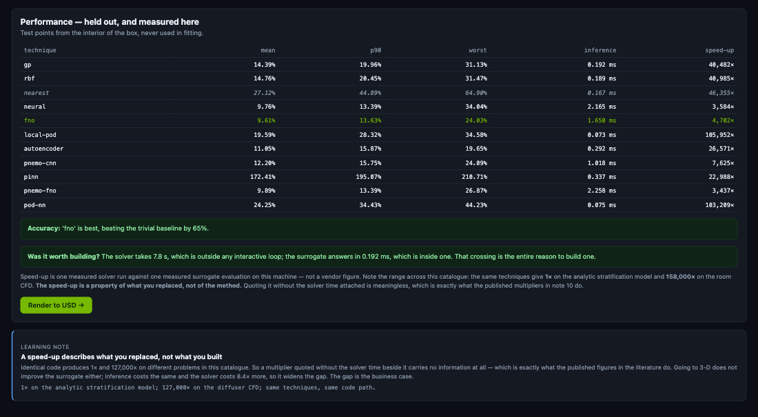
The moving-diffuser run is the closest contest in the 2D set: the hand-written FNO, the PhysicsNeMo FNO and a plain neural field model land within 0.28 percentage points, while POD-NN falls well behind. One winner label hides a cluster of methods and a much larger tail error.
A better regressor helped without replacing the basis
My original reasoning was simple. If projection error is already below 1%, changing the representation can’t recover much. I took that to mean the neural methods had little room to help.
I had bounded the wrong thing: projection error says what a better basis could recover, but it says nothing about what a better regressor could recover when regression carries nearly all the error.
POD-NN became the useful control. It uses the same POD basis and the same modal coefficients as POD+GP. The change is in the map from inputs to coefficients: the Gaussian-process path predicts each coefficient independently, while POD-NN predicts them jointly through a small shared network.
It reduced the ventilated-room mean from 8.10% to 5.00% and the energy case from 2.78% to 1.22% without changing the representation. That is evidence that regression capacity mattered on those problems.
It didn’t work everywhere. The moving-diffuser dataset retained 65 modes from 120 training snapshots, only 1.8 snapshots for each coefficient being predicted. POD-NN reached 24.25%, far behind POD+GP at 14.39% and FNO at 9.61%. That result is consistent with an overfit joint regressor when the reduced problem was thinly supported. I would use it as a direction to test, not as a diagnosis or threshold.
Changing the basis did help, just not for the reason I expected
The direct FNO path won stratification, contaminant dispersion and the moving diffuser. NVIDIA PhysicsNeMo’s FNO implementation landed within 0.14 to 1.21 percentage points of the hand-written FNO across the four problems in the common catalogue run. That agreement increased my confidence that the architecture contributed to the result. It isn’t proof: both paths share data, preprocessing and possible implementation biases.
The result still needs problem-specific reading.
The moving diffuser changes the supply location, so the field feature moves across the grid. The result is consistent with a fixed global basis spending modes on those shifted states. FNO works on the field directly and was the best of the tested implementations, although its advantage over the other neural field models was less than one point.
I included contaminant dispersion because I expected a moving plume to be difficult for linear compression. FNO did win, but the case itself didn’t test what I intended. First-order upwind advection in the demonstration solver added enough numerical diffusion to smooth the plume. The solver made the output easier to compress before any surrogate saw it. I can’t use that result to claim that FNO handles a sharp contaminant front; it shows how a low-fidelity reference can erase the feature a benchmark was built to test.
The stratification case is analytic and its reference evaluation takes about 0.02 milliseconds. FNO’s 0.12% error is impressive and operationally irrelevant: the direct calculation is already fast. Part 1’s first gate rejects the surrogate before model selection starts.
The same caution applies to the small differences in the catalogue: neural fitting is stochastic, this study doesn’t yet carry a multi-seed distribution for every model, and a 0.28-point gap among the leading moving-diffuser models is a prompt for another run rather than a durable ranking.
Two failures made the diagnosis clearer
Local POD was meant to help when one global linear basis could not span the solution family. It won none of the four problems in the complete catalogue run. On the moving diffuser, the global POD+GP result was 14.39%; splitting the parameter space into local bases moved it to 19.59%.
That is what I should expect when representation is already good and regression is starved of data, because partitioning gives each local regressor fewer snapshots while addressing a basis problem the projection test did not find.
The physics-informed network scored between 84% and 172% in the four-problem catalogue run. On two problems it was worse than predicting zero everywhere. This isn’t a verdict on physics-informed learning as a field. It is a verdict on using this small PINN implementation and training setup as a fast forward surrogate for these parameter-to-field tasks. Adding a residual term didn’t make sparse supervision disappear, and the result didn’t earn a place in the runtime path.
I kept both rows. A comparison that drops the methods that failed would turn the workbench into a product demo.
The room result changed when I scored the decision
The 5.00% POD-NN result makes it the whole-field winner on the 2D ventilated room, but the ordering changed when I re-scored all 26 held-out fields on occupied-zone temperature, air speed and vertical gradient. POD-NN even fell behind the nearest-snapshot baseline on the gradient. Part 5 owns that table and what it means for a comfort loop; here it is the boundary on the 2D technique ranking.
What the 2D work changed
I came into these runs expecting the method choice to follow the spectrum: slow decay would point me toward a nonlinear model or neural operator, while fast decay would justify POD+GP. The projection measurements showed fast enough decay and a usable basis almost everywhere. The results then separated on the regression and the data.
These runs changed where I spend the next experiment. Once a surrogate is justified, I measure projection error before reaching for a different representation: low projection sends me toward denser samples and another regressor, while high projection earns a test of the basis itself. In both cases I keep the nearest baseline and the failed rows, because they expose problems that a winner-only table hides.
Part 4 moves the same question into 3D. The output gets larger, the reference solver changes, the small test set changes the apparent winner, and model size becomes part of the choice.
Disclaimer: The views and opinions expressed in this account are those of my own and do not represent those of my employer, NVIDIA.