When Does a Digital Twin Need a Surrogate?

I’ve seen a digital-twin project begin as a top priority, complete its pilot, and then face a much harder question when the team tried to scale it: what additional value would the next site or line receive? The pilot had made plant information easier to see, which was useful because the existing experience was poor. Much of the same information had already been available through dashboards and reports, however, so the scale decision needed more than easier access.

That experience is why I ask what the twin lets someone decide. Showing the current state is useful. Comparing changes before anyone makes them asks more of the model: it has to predict alternatives while there is still time to act. I then need to know whether the original solver can answer quickly enough for that decision.

I chose ventilation and comfort to examine that question. A building management system may already expose zone temperatures, equipment state, alarms and energy data. Local airflow and temperature predictions could help a facilities engineer compare operating choices that those existing views do not resolve.

A ventilated room makes it concrete. A facilities engineer may want to know whether people near a window will be uncomfortable under the current weather and occupancy. A computational fluid dynamics solver can estimate the temperature and airflow fields. If the question is asked once during design, waiting for that solve may be entirely reasonable.

The operational question is different:

• What happens if the supply temperature changes?
• Would moving more air remove the warm region without creating draft below the diffuser?
• Which of twenty control choices gives the best comfort with an acceptable energy cost?
• Does the answer change when occupancy or solar load changes?

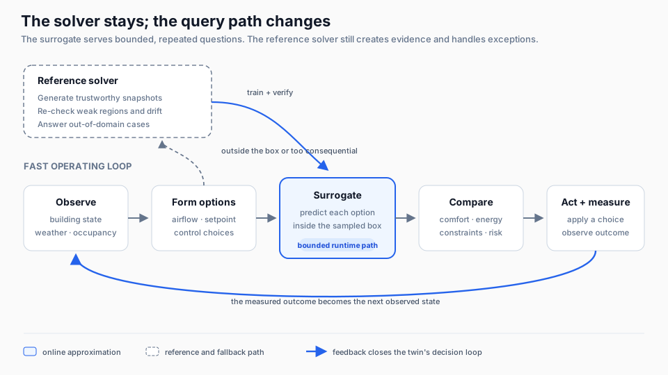
Each candidate needs another prediction. If those solves take longer than the engineer has to decide, I would test a surrogate: a bounded approximation learned from results the solver has already produced. It can make repeated queries faster while the original solver remains the reference for checking them.

I thought this would become a general case for surrogate modeling. Then the energy and analytic cases in the workbench showed me calculations that could already fit the decision window. Adding a learned approximation there would create training and validation work without necessarily saving time the application needed. I now measure that workload before choosing an algorithm.

The loop sets the latency requirement

Simulation occupies the prediction step in this loop. I had reached the same conclusion from visual twins: the decision determines what kind of truth the twin needs. The twin supplies the surrounding context: current state, asset identity, constraints, the action being considered and a way to compare the prediction with what happens next.

The acceptable latency comes from that loop: an overnight planning study, a design review, a control-room what-if tool and an automatic controller don’t have the same time budget, and calling all four “runtime” hides the design decision that matters.

I use one question as the first gate:

What is waiting for the solver?

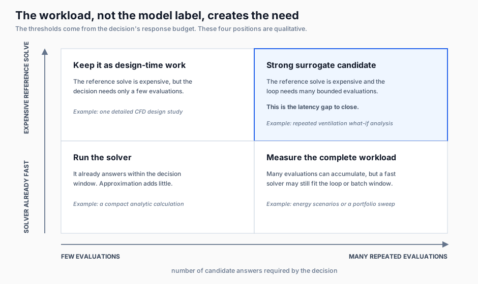
If the answer is nothing, I keep the solver. A model that is already fast enough for the required number of evaluations has no latency problem to solve. Replacing it with a surrogate would add training data, validation and out-of-domain risk while removing direct access to the original equations.

If a person is waiting for every answer, an optimizer needs thousands of evaluations or a control application has a firm response window, the arithmetic can change quickly. The cost that matters is not one solve in isolation. It is:

solver time × candidates × operating conditions × times the decision repeats

I use that workload rather than the name of the solver to decide what to test next.

What is waiting changes across the stack

In the industrial systems I know, “what is waiting for the solver?” has at least three answers. They sit roughly at the field, control and operations layers of the ISA-95 stack I use in my MES work, but the more useful distinction is who or what has to decide and how long it can wait.

The field-layer case isn’t hypothetical for me. In predictive emissions monitoring work, a physical analyzer in a hot, corrosive stack was expensive to keep healthy, so the model inferred emissions from fuel flow, oxygen, load and temperature. Nobody waited for a recommendation at that layer; the model became the reading, and an out-of-range result started a written procedure.

I saw the control-layer version in Pavilion8 advanced process control. We identified a process model from plant tests, gave it a prediction horizon and constraints, and let the controller choose the next move inside a fixed response window while the operator supervised the envelope. Plant safety remained in separate layers because the model could be wrong.

At the lower layer, software may consume the answer automatically. At the MES layer, a person may be comparing choices before the shift or schedule moves on. The same solver time can be acceptable at one layer and unusable at another because the decider, consequence and clock have changed.

I don’t think crossing into this kind of decision support is as inaccessible as it first looks. The domain handoff is learnable; the modeling and validation aren’t easy. A reference solver can be wrong or fail to settle, an operating box can cross into another regime, a small test can flatter one model, and a learned path can get worse when the setup changes. The rest of this series contains every one of those failures. The industrial team already knows the decision, constraints, timing and consequence; the simulation work supplies a reference model, and the surrogate earns a role only if it can connect the two within a tested boundary.

Ventilation makes the distinction visible

Ventilation and thermal comfort are a useful running case because the decision depends on spatial effects.

A whole-building energy model can estimate loads, equipment response and zone conditions. For many uses, that is exactly the right model, and it may already run quickly enough. But a conventional one-node zone average cannot tell me that one person is sitting in the supply jet while another is beside warm glazing. Those questions need local temperature and velocity, and sometimes turbulence and radiant conditions as well.

CFD can provide the missing fields. It can also be expensive enough that exploring many control settings becomes awkward. A surrogate built over a deliberately narrow operating range can make that local prediction available to the decision layer without pretending that CFD has become instantaneous.

The arrangement I have in mind is not “AI replaces simulation.” CFD or another first-principles solver establishes the reference response. The surrogate explores bounded alternatives. Comfort, energy or operating criteria turn those fields into something a user can act on. Fresh solver runs and observed building data check weak regions and drift.

The surrogate is one execution path within the twin. I still need the full solver for new geometry, operating regimes outside the sampled range, periodic verification and any case where the approximation is not good enough for the consequence of the decision.

This distinction also prevents a common error: reporting a low whole-field error and treating it as proof that the comfort decision is correct. An average error across every grid cell can hide a larger error at occupied height or near a diffuser. A model intended for comfort has to be assessed on comfort-relevant quantities and locations, not only on the field as a whole.

Energy is the useful counterexample

Energy is often the first use case proposed for a building surrogate. Sometimes that makes sense. A portfolio optimizer may need to evaluate many buildings, many retrofit combinations and many weather scenarios. Even a relatively fast energy model can become the bottleneck when the loop multiplies its cost enough times.

But the word energy doesn’t make a surrogate necessary. If the task is a nightly calculation, a small scenario set or a model that already returns within the application’s response budget, the solver itself may be the better runtime model.

The energy case left me with a narrower rule:

Use a surrogate when the complete decision workload is too slow, not merely because the underlying method is called a solver.

Solver acceleration is another valid option. A reduced discretisation, a different numerical method, parallel hardware or a GPU implementation may close the latency gap without creating a learned approximation. If the accelerated solver meets the loop’s budget, it retains an important advantage: it is still computing the modeled physics for the new input.

I would choose the smallest trustworthy model that meets the decision’s latency, fidelity and operating-domain requirements. Sometimes that remains the solver.

Surrogate and ROM are not competing categories

I originally treated a reduced-order model, or ROM, and a surrogate as competing choices. They describe different things: a surrogate stands in for a more expensive mapping, while a ROM reduces the degrees of freedom in a model. A reduced representation with a learned parameter map can be both.

Once the workload justifies an approximation, I compare concrete implementations and their assumptions. The workbench article explains the reduced models, regressors and neural operators used in this series. Their names do not settle whether the application needs any of them.

Why 2D and 3D both belong in the study

I use the cheaper 2D cases to debug the comparisons, then ask whether the findings survive a 3D problem closer to the intended use. The move changes the reference solver, spatial behavior and model costs. A 2D winner is evidence about that test, and even the 3D demonstration solver still needs validation before its output can support an engineering comfort claim.

Five gates before putting a surrogate in the loop

Before choosing a technique, I would want five questions answered.

1. Is latency actually blocking the decision? Measure the solver against the complete number of evaluations and the loop’s response budget. Include fast-solver and solver-acceleration options.
2. Can the operating domain be bounded? Inputs, ranges, geometry and regimes have to be explicit. “Any room under any condition” is not a tractable parameter box.
3. Can trustworthy reference data be generated? The training budget is primarily a solver-run budget. Non-converged or otherwise invalid runs can’t become reliable ground truth by being passed to a learning algorithm.
4. Is accuracy measured on the decision? Use held-out conditions and include the quantities that determine the action: local comfort, energy, constraint violations or another relevant outcome, not only an aggregate field score.
5. Is there a safe path outside the model’s competence? Enforce the parameter box, identify weak regions, retain the solver and route uncertain or consequential cases back to it.

Only after those gates does model selection become the main question.

From argument to measured comparison

I am building SurrogateGate to make this choice empirical. Part 2 introduces SurrogateLab, the executable workbench and report layer behind the project. It compares classical reduced models, neural regressors, neural operators and PhysicsNeMo implementations across contrasting 2D and 3D datasets.

The aim isn’t to produce one leaderboard winner. It is to identify the conditions under which different techniques win, fail or never need to be built in the first place.

Part 3 follows the techniques across five 2D problems, Part 4 rebuilds the 3D comparison on a common test set, and Part 5 returns to the ventilated room as an operational comfort case.

Disclaimer: The views and opinions expressed in this account are those of my own and do not represent those of my employer, NVIDIA.